One common approach to toon/NPR outlines is to locate contours by inspecting G-buffer data — comparing depth, normal, and/or object-ID samples between neighboring pixels and flagging an edge wherever the discontinuity crosses some threshold. This is different from geometry-based approaches like inverted hull, which draw the outline as an actual mesh and don’t have the problem described below — they’re inherently TAA-compatible. G-buffer-based detection works well without a temporal upscaler, but runs into a subtle problem once one — TAAU, DLSS, FSR2, XeSS, Unreal’s TSR, and similar — is added to the pipeline.

These upscalers render the scene at a reduced internal resolution (the screen percentage, or render scale) and reconstruct a full display-resolution image from it using temporal accumulation. A G-buffer contour algorithm, at its core, is just an edge detector: for a given render-resolution pixel, it answers “does a contour pass through this pixel?” or “does a contour pass between these two pixels?”

Since the G-buffer only has samples at render resolution, the thinnest outline such an algorithm can ever produce is exactly one render pixel wide — there is no sub-pixel information to draw anything thinner from.

That constraint becomes visible the moment the image is upscaled. If the renderer runs at 50% screen percentage, the upscaler doubles the linear dimensions when reconstructing the display-resolution frame. A contour that was already at the minimum representable width of one render pixel gets stretched along with everything else, and comes out at roughly 1 / screen_percentage display pixels wide — two display pixels at 50% screen percentage, four at 25%, and so on:

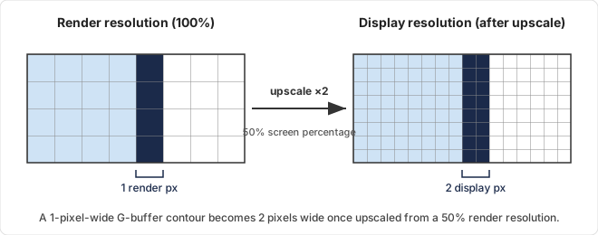
In other words, the thinnest outline the algorithm can draw gets thicker, in display pixels, as render resolution drops relative to display resolution — the opposite of what you’d want from an outline style that’s supposed to stay crisp and resolution-independent.

A simple, standard compromise is to blur the render-resolution outline by an amount that scales with the screen percentage, or to supersample the depth and normal G-buffer data. Now, in this post, I’m proposing an algorithm that keeps the outline crisp without those trade-offs — see below for the core idea.

How Do Temporal Upscalers Reconstruct Sub-Render-Pixel Detail

Temporal upscalers don’t get extra detail from any single frame — a single frame is still only rendered, and G-buffer-sampled, at render resolution. What they add is time.

Each frame, the camera’s projection is offset by a small sub-pixel jitter — typically a low-discrepancy sequence like a Halton sequence, cycling through a handful of offsets that together cover the pixel footprint fairly evenly. So frame N samples the scene at one sub-pixel position within each render pixel, frame N+1 samples it at a different sub-pixel position, and so on. The upscaler then reprojects previous frames into the current frame using per-pixel motion vectors and blends them with the current frame’s jittered sample into a history buffer. After a handful of frames, that history buffer holds several samples per render pixel — this jitter-and-accumulate loop is basically how temporal upscalers scan out sub-render-pixel detail over time, rather than any single frame having more resolution than the G-buffer it was built from.

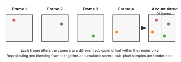
This is why geometry-based outline techniques like inverted hull don’t have the thickness problem described above: an outline mesh is rasterized like any other triangle in the scene, at whatever jittered sub-pixel offset that frame happens to use. Its silhouette edge lands at a slightly different sub-pixel position each frame, gets accumulated the same way ordinary geometry edges do, and comes out anti-aliased and sub-render-pixel-accurate after temporal accumulation — with no extra work.

A G-buffer contour detector doesn’t get that benefit for free. Even though the underlying G-buffer samples are taken at a jittered sub-pixel offset each frame, the detector’s output — is there a contour here, yes or no — is still a value computed once per render pixel, on a fixed pixel grid. There’s no continuous edge for the accumulation to refine the position of; the history buffer just receives four frames’ worth of “yes, this pixel is on a contour,” instead of four different sub-pixel edge positions the way a rasterized triangle edge would produce. That mismatch — a discrete, grid-locked detector feeding into a system built to accumulate continuous sub-pixel geometry — is the root of the pixel-thickness problem.

Core Idea

The Goal: Reconstruct the Edge, Not Just Detect It

Everything above treats the G-buffer algorithm as a binary detector: does a contour cross this one-render-pixel-long segment, yes or no. The goal of this algorithm is to go a step further and reconstruct the actual line-segment equation of the edge or contour near each render pixel, instead of just detecting whether one exists. Concretely, the edge is reconstructed as $x = a + by$ in that pixel’s local space — coordinates measured relative to the render pixel itself, rather than screen space — which is also the form the OLS fit further down solves for.

Once you have that line equation, rendering the outline becomes a distance check: draw the outline at a render pixel only when the distance from that pixel’s jittered sample position to the reconstructed edge line falls within some desired thickness. Because that threshold is a property of the reconstructed edge rather than of the render-pixel grid, it can be set arbitrarily thin — even below the display pixel’s width — and it stays consistent regardless of the upscaler’s screen percentage. That’s the sub-render-pixel-accurate, TAA-compatible outline this post opened with.

What G-Buffer Algorithms Do

Take a really simple G-buffer algorithm as an example. For a given target pixel, it checks whether the depth or normal value differs from each of its four axial neighbors — up, down, left, right — by more than some threshold. If the difference exceeds the threshold against any one of those neighbors, the target pixel is marked as containing an outline.

Marking both sides of every discontinuity like this produces an outline that’s two render pixels thick. You can narrow that down to one render pixel by only drawing the outline on whichever side of the pair has the higher depth (i.e. is farther from the camera), or the more camera-facing normal.

Here’s the important part: what the algorithm is actually doing is checking whether an edge exists between the jittered sample positions of the target pixel and each neighbor — not between the pixels’ centers or their full footprints. So, effectively, it’s detecting whether an edge crosses the one-render-pixel-long line segment connecting the target’s jittered sample to that neighbor’s jittered sample, because G-buffer data is collected from the jittering positions.

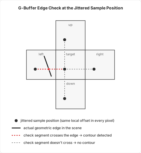
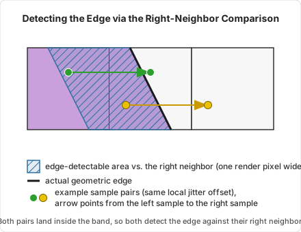
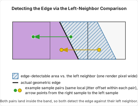
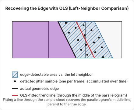
So, given an actual geometric edge — the line along which the real discontinuity occurs — the set of jitter offsets that would place it between two neighboring pixels forms a parallelogram: two render pixels wide, running parallel to the edge, with the edge itself as its middle line. If the jitter offset for that frame falls inside this parallelogram, the edge is detected between the two pixels; otherwise, it isn’t.

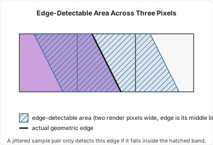
Let’s ignore the top and bottom comparisons of the G-buffer algorithm and just look at the left and right neighbor comparisons. The edge line segment splits the parallelogram into two one-pixel-wide halves: the left half detects the edge when a pixel’s jittered sample is compared with its right neighbor, and the right half detects it when compared with its left neighbor.

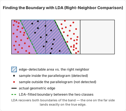
The same thing holds on the other side, mirrored: the right half of the parallelogram is the region where a pixel’s jittered sample detects the edge against its left neighbor.

And, just as important, here’s what it looks like when the edge isn’t detected: when a pair’s shared jitter offset falls outside the band, both samples land on the same surface, so the comparison finds no discontinuity at all.

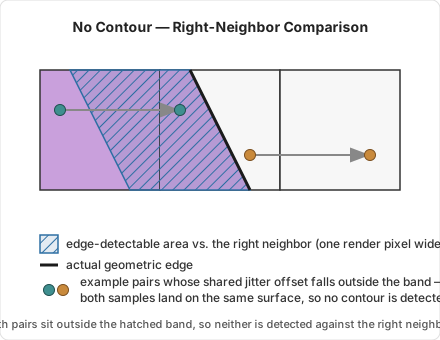
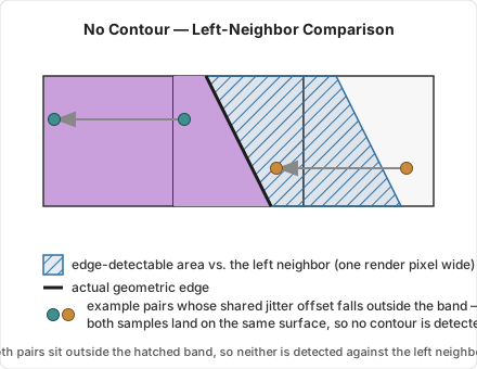
So, for each neighbor-comparison direction, the detected/not-detected jitter samples accumulated across many frames give you the data to infer the shape of that direction’s parallelogram.

Using Statistical Methods with a Temporal Record

You can fit that data with a statistical method like ordinary least squares regression to find the line running through the middle of the detected samples, or linear discriminant analysis to find the boundary between the detected and not-detected samples instead. Either way, you end up with an estimate of the edge’s position and orientation that’s noticeably more accurate than any single frame’s one-pixel-wide detection.

LDA takes a different approach: instead of fitting through the middle of one class, it looks for the boundary that best separates two labeled classes of points. Label each accumulated jitter sample by whether that frame’s comparison detected a contour or not, and LDA gives you back the line that best separates the “detected” cluster from the “not detected” one. Since the detectable band has two sides, running this twice — once against the samples just outside its near edge, once against the samples just outside its far edge — recovers both boundaries of the band. One of those boundaries is, by construction, the true geometric edge itself.

This sounds nice, but it seems like you’d need to hold onto every sampled point to compute either statistic. Actually, you don’t — both OLS and LDA can be computed from a handful of running sums, so you can apply them to data that’s accumulated temporally, with decay, instead of keeping every sample around.

Ex. OLS with Temporal Accumulation

As a quick illustration of that pattern, here’s what it looks like for OLS specifically — I’ll go into the full implementation, as a dedicated section of its own, later in this post.

Given accumulated samples $(x_i, y_i)$, OLS fits the line $x = a + by$ using only four running statistics — $E[x]$, $E[y]$, $E[y^2]$, and $E[xy]$ — each of which can be maintained as a decayed running average, updated by one new sample per frame:

And each of those four expectations can be maintained without needing to store any history, by keeping a single decayed running value per variable and updating it once per frame:

where $v_i$ is that frame’s new sample for whichever variable — $x$, $y$, $y^2$, or $xy$ — and $d \in (0,1)$ is the decay rate. After enough frames, $\langle v \rangle_i$ tracks $E[v]$ closely enough to plug directly into the OLS formula above.

Actual Implementation with Temporal OLS

1st Approach, Using edge detected points

Each render pixel maintains a historically accumulated record of the required data for each of its four edge-inducing directions (top, bottom, left, right). Each record holds the four running statistics the fit needs — $\langle x\rangle$, $\langle y\rangle$, $\langle y^2\rangle$, $\langle xy\rangle$ — plus $\langle x^2\rangle$ and a decayed sample count $n$, which the Edge Selection section uses to measure how reliable each fit is. Each statistic is stored as a single float4, one component per inducer direction.

The first problem I ran into was that the sampled data gets cut off at the pixel boundary.

For a given inducer direction, an edge produces edge-detected jitter positions across two pixels: the pixel that actually contains the edge, and the pixel on the opposite side from the inducer direction.

Once you know which of the two is the containing pixel, you can simply merge the other pixel’s data into it. This is doable as long as the edge is isolated — no other edge within a radius of two render pixels. For each inducer direction, you just check whether the neighboring pixel in that direction also has data for the same inducer direction.

However, what if two edges are less than two render pixels apart? This would leave more than two consecutive pixels holding left-induced edge data.

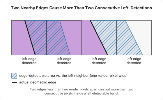
Well, the solution turns out to be simple: don’t merge neighboring pixels’ data at all. Instead, apply OLS to each render pixel independently, using only the data built from that pixel’s own jitter samples.

This yields a line that runs not through the middle of the full parallelogram, but through the middle of the trapezoid formed by cutting that parallelogram at the pixel boundary.

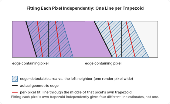
Even so, assuming the accumulated data is accurate enough, you can reconstruct the true edge segment from these per-pixel fits.

A pixel that doesn’t contain the actual edge will always have an intercept less than 0.5, so checking the intercept alone tells you whether a given pixel contains the edge or not.

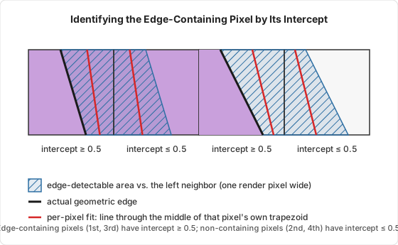
For the edge-containing pixel, you’re left with the line equation that runs through the middle of its trapezoid — and from there, simple algebra reconstructs the actual edge equation.

Work in local pixel coordinates, $x, y \in [0, 1]$, and parametrize the edge as $x = A + By$ rather than $y = A + Bx$ — every edge in this post enters through the top of its pixel and exits through the bottom, so solving for $x$ as a function of $y$ avoids the near-vertical slope that form would otherwise have. For the edge-containing pixel, the left trapezoid is the region $0 \le x \le A + By$, so at each height $y$ its horizontal slice runs from $0$ to $A + By$, and the midpoint of that slice is $(A+By)/2$. The line through the middle of the trapezoid is exactly the line through all of those midpoints:

So if $x = a + by$ is the line through the middle of the trapezoid, the actual edge is just that line doubled:

2nd Approach, Using both edge detected and not detected points

For each inducer direction, the 1st approach only accumulates jitter samples that detected the edge, and discards the ones that didn’t. But those discarded points still carry information about the edge-not-detected region — just throwing them away is a waste.

Take the right-inducer check on a pixel that contains an edge: it detects the edge inside the left trapezoid, $0 \le x \le A+By$. The frames where that comparison came back negative are exactly the pixel’s complementary region, the right trapezoid $A+By \le x \le 1$. You can accumulate the same running statistics from those not-detected samples and fit them with OLS the same way, giving a line $x = a_{nd} + b_{nd}y$ through the middle of that not-detected trapezoid. At height $y$, its horizontal slice runs from $A+By$ to $1$, so its midpoint is $\big((A+By)+1\big)/2 = \tfrac12 + a + by$ — the detected trapezoid’s own midline, shifted right by a constant half pixel:

So the not-detected samples recover the same edge, once you undo that fixed shift and double the result the same way as before: $A = 2(a_{nd}-\tfrac12)$, $B = 2b_{nd}$.

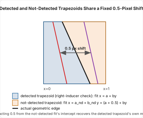
However, you don’t need two independent estimates of the same edge for one inducer direction. For a given direction, if a sample didn’t detect the edge via that direction’s own check but did detect it via the opposite direction’s check, shift that sample 0.5 pixels the opposite way and accumulate it straight into the same running sums, as if it were one of that direction’s own detected points.

For example, take the right-inducer estimator: if a sample failed to detect the edge against the right neighbor but did detect it against the left neighbor, shift the sample 0.5 pixels to the left and fold it into the right-inducer’s running sums.

This works because, for the pixel that actually contains the edge, a not-detected sample for one direction’s check is, at the same time, a detected sample for the opposite direction’s check. Take a vertical edge and just the left and right inducer checks: a jitter sample at local position $x$ triggers the right-inducer check whenever $x \le A+By$, and the left-inducer check whenever $x \ge A+By$ — complementary conditions, ignoring the boundary itself. So “not detected by the right-inducer check” and “detected by the left-inducer check” describe the same set of samples.

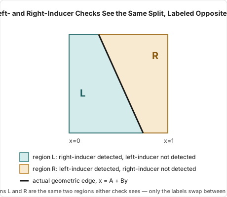
A sample that detects the edge in neither direction still gets discarded, same as in the 1st approach — you’re not accumulating a point for every single frame, only for frames where one of the two checks actually fires. That’s worth doing on purpose, not just for accuracy: if a pixel far from any edge started accumulating “nothing detected” data too, it would become statistically hard to tell apart from a pixel that sits right next to an edge but simply missed it on a given frame. Leaving the accumulator untouched when neither check fires keeps the sample count itself a meaningful signal — pixels near an edge build up real data quickly, pixels nowhere near one stay empty.

Which means you don’t need four direction accumulators. Pick one direction per axis — right for the horizontal axis, top for the vertical, say — and you already have both halves of what you need: that direction’s own detected samples, and the opposite direction’s detected samples doing double duty as its not-detected samples, via the same 0.5 shift above. The other two accumulators can be dropped.

Fully Using Both Parallelograms’ Data

This same-axis merge also means the algorithm ends up using the full data of both parallelograms next to the pixel, not just half of each.

Consider a single edge inside pixel B, with left and right neighbors A and C. Along the horizontal axis, there are two parallelograms that can detect this edge: one straddling the A–B boundary, and one straddling the B–C boundary — together they’re just the usual single parallelogram from earlier, split down the middle by the true edge.

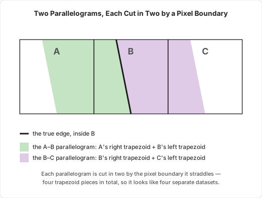
Each parallelogram is cut in two by the pixel boundary it straddles, so there are four trapezoid regions in total: A’s right trapezoid and B’s left trapezoid make up the A–B parallelogram, while B’s right trapezoid and C’s left trapezoid make up the B–C parallelogram. That looks like four separate datasets to keep track of.

It’s actually only two — just not the two you’d guess from the picture above.

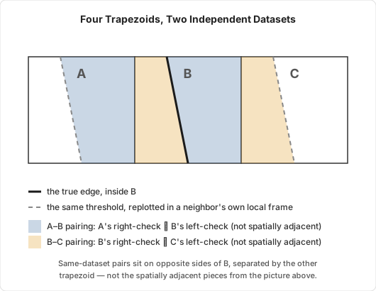
A’s right trapezoid has exactly the same shape as B’s right trapezoid. The same is true for C’s left trapezoid and B’s left trapezoid. Remember, we detect an edge by comparing two jittering positions in two neighboring pixels.

For example, say in one frame the jittering position hits the right trapezoid in pixel B — then it also hits the same-shaped right trapezoid in pixel A. B’s left-inducer check returns true from that two-point comparison, and A’s right-inducer check returns true from the exact same comparison.

So the axial merge makes full use of both parallelograms’ data — none of it is discarded, not even the portion that falls outside the edge-containing pixel.

Co-trigger Points

This only holds while a single edge crosses the pixel along that axis, though. Once there are two — say a sliver of a third surface, narrower than one pixel, sitting between them — a sample landing inside that sliver can trigger both the left- and right-inducer checks in the same frame, since it disagrees with both neighbors at once.

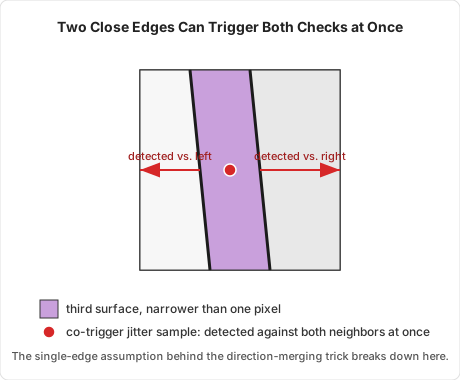
I keep a decayed running count of these co-trigger events per axis, next to the running sums, and treat the ratio of co-trigger frames to total accumulated frames as a reliability signal. When that ratio runs high, the merge’s single-edge assumption no longer holds.

If both the horizontal and vertical axis estimates are unreliable for a pixel, the simplest fix is to just not draw an outline on it at all. Such a pixel is dense with same-axis edges, which often causes flickering anyway.

Flickering is one of the outline’s persistent issues — I’ll cover how I handle it in a later section.

3rd Approach, Fixing the Dashed-Line Artifact

The Problem With the 2nd Approach

The 2nd approach made the edge converge faster, but it introduced an unexpected artifact: when the true edge sits close to a pixel boundary, statistical noise can make a pixel conclude it doesn’t contain the edge, and assume a neighbor does instead.

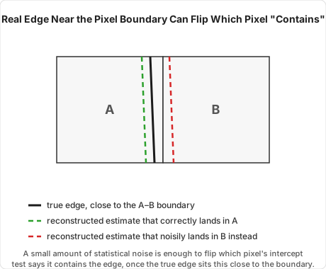
This wasn’t a problem in the 1st approach, because neighboring pixels were working from the same underlying data. Say there are two horizontally adjacent pixels, A and B, with a nearly vertical edge inside A, close to the A–B boundary. If A’s right inducer check wrongly concluded that B contains the edge, the corresponding B’s left inducer check would reach the same wrong conclusion that B contains the edge in the 1st approach too — the outline stayed a single, consistent pixel wide, just possibly the wrong one.

With the 2nd approach, though, A and B can each go wrong independently.

Consider only the horizontal-inducer case, with a nearly vertical edge — and bring in the third pixel, C, B’s neighbor on the other side. As established above, a vertical edge gives two datasets, L1 and R1, inside the edge-containing pixel B. The left neighbor, A, holds a shifted copy of R1 — call it R2. The right neighbor, C, holds a shifted copy of L1 — call it L2. The edge-containing pixel, B, draws on both L1 and R1. Each neighbor, since it doesn’t actually contain the edge, only has access to one of R2 or L2 — never both.

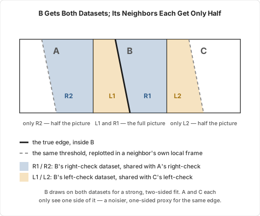
That asymmetry is the root cause: B gets a strong, two-sided fit, while A and C each only get a noisier, one-sided proxy for the same edge. So A and C can land on the wrong side of the containment test independently of each other — both may conclude they contain the edge, or both may conclude they don’t. That produces a dashed outline — the contour repeatedly thickens to two pixels or drops out entirely, instead of staying a clean, consistent pixel wide.

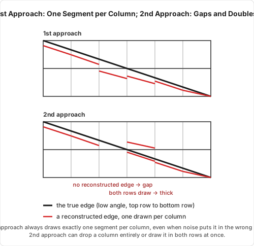
A mostly-horizontal edge repeats this same gap-or-thickness pattern as it crosses row after row of pixels, producing the dashed-outline artifact.

Solution

The fix is to make neighboring pixels fit exactly the same data. The key observation is that the edge-containing pixel’s own record is already duplicated, piece by piece, in its two neighbors: B holds L1 and R1, A holds a copy of R1, and C holds a copy of L1. So instead of fitting its own estimator, each pixel fits the combination of its two neighbors’ estimators along the same axis — the left and right neighbors for the horizontally induced edge, the top and bottom neighbors for the vertical one. This needs a decayed running sample count for each pixel too, so each neighbor’s contribution can be weighted by how much data it actually has.

Every pixel stores its running statistics in its own local coordinates, though, so a neighbor’s statistics first need to be shifted into the reading pixel’s frame. Take the horizontal-inducer case as the example, keeping the left inducer as the axis’s kept direction this time. As before, the edge inside B splits it into L1 and R1, the left neighbor A holds R2, and the right neighbor C holds L2.

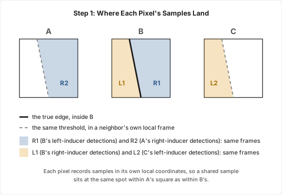
Each pixel folds its own samples into its left-inducer estimator. For B, R1 samples are left-inducer detections, so they’re kept as they are, while L1 samples are right-inducer detections, so they’re shifted 0.5 pixels right first, landing on top of R1. A’s R2 samples are right-inducer detections from A’s point of view, so A shifts them 0.5 pixels right too, which pushes them past A’s own right boundary. C’s L2 samples are left-inducer detections from C’s point of view, so C keeps them as they are.

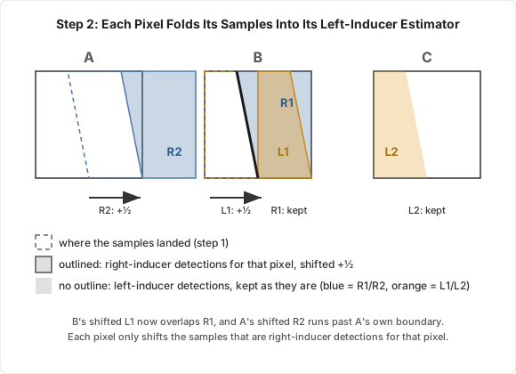
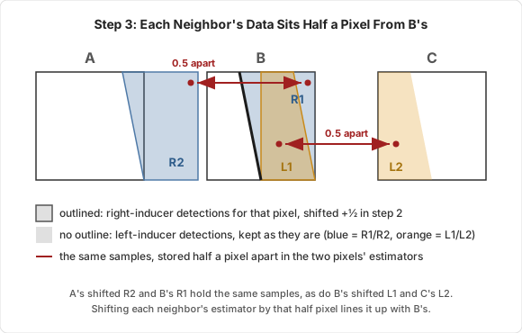
Now compare what each pixel ended up storing. A’s right-inducer check fires on exactly the same frames as B’s left-inducer check, since they’re the same comparison, and at the same local jitter position $x$, since every pixel shares the jitter offset. B kept those samples where they were, but A shifted them half a pixel right, so for every sample they share, A’s stored $x$ is exactly half a pixel greater than B’s. Shifting A’s statistics by $-\tfrac12$ lays them right on top of R1. C mirrors this: C’s L2 samples are the same frames as B’s L1, which B shifted half a pixel right and C didn’t, so C’s statistics shift by $+\tfrac12$ to land on B’s shifted L1, which itself overlaps R1.

Expanding $x’ = x - \tfrac12$ inside each of A’s running averages, the same substitution used earlier for the not-detected trapezoid, gives:

and $x’ = x + \tfrac12$ for C:

$\langle y\rangle$ and $\langle y^2\rangle$ don’t need shifting, since A, B, and C share the same vertical extent. The rule is the same from any pixel’s point of view: a neighbor one pixel to the left is shifted by $-\tfrac12$, and a neighbor one pixel to the right by $+\tfrac12$.

The shift is half a pixel, even though the neighbors sit a full pixel away. The estimators don’t store raw geometric positions. They store positions folded into each pixel’s own trapezoid, and one side of that trapezoid is pinned to the pixel’s own boundary, so moving the edge by a whole pixel moves the trapezoid’s midline by only half. The same $\mp\tfrac12$ comes out if the right inducer is kept instead: every pixel’s own shifts flip direction together, so the difference between them stays the same.

With both neighbors’ statistics expressed in B’s frame, B’s fit is their weighted average, using each neighbor’s decayed sample count $n$ as the weight:

Now look at what each of the three pixels ends up fitting:

• B fits A’s R2 and C’s L2, which are the same samples as R1 and L1: $R1 \cup L1$.
• A fits its own left neighbor and B. A’s left neighbor holds nothing from this edge, since none of its pairs straddle it, so A fits B’s record: $L1 \cup R1$.
• C, by the mirror argument, fits B’s record: $L1 \cup R1$.

All three fit the same samples, only expressed in their own coordinates, so they decode the same line and agree on exactly which pixel contains it. That’s the guarantee the 1st approach had, now with the 2nd approach’s doubled sample count. The fitted statistics then go straight into the same OLS formula used everywhere else in this post.

Why Leave Out a Pixel’s Own Data

It might seem natural to pool each pixel’s own record together with its neighbors’ instead of dropping it. That gives:

The three pixels no longer fit the same data: A counts R1 twice, and C counts L1 twice. That difference looks harmless, because the dashed-line artifact only shows up when the edge sits close to a pixel boundary, and there one of the two trapezoids is only a sliver. With the edge near B’s left boundary, for example, L1 holds very few samples, so B’s $L1 \cup R1$ and A’s $L1 \cup 2R1$ differ only in how much weight that sliver gets.

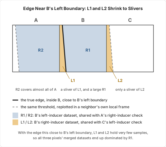
But that’s exactly the case where the decision between A and B is on a knife edge. The edge is only a sliver’s width away from their shared boundary, so the margin either fit has to stay on the right side of is just as small as the data difference between them. A small difference is enough to push A and B to different conclusions, and the gaps and doubles come back. Dropping the pixel’s own record removes the difference entirely.

Falling Back When Neighbors Are Unreliable

Fitting only the neighbors assumes their records describe this edge alone. A neighbor with a high co-trigger ratio (see Co-trigger Points) has samples from a second edge mixed into its record, and fitting it would pull B’s line off. In that case B switches to its own record entirely:

where $\rho_A$ and $\rho_C$ are the neighbors’ co-trigger ratios and $\tau_\rho$ is a threshold. A neighbor with no samples contributes nothing and doesn’t trigger the switch, and when neither neighbor has any samples, B uses its own record too.

The switch is all or nothing on purpose, rather than a blend weighted by the co-trigger ratio. When the pixel that falls back is the edge-containing one, its own record is exactly the $L1 \cup R1$ its neighbors would have supplied, so nothing is lost. A blend, on the other hand, gives one pixel a mix of its own record and its neighbors’ while the pixel next to it still fits unmixed data, which brings back a partial version of the mismatch from the previous section. The pixels where the switch fires are the dense-edge ones that already tend to flicker, and that get culled when both axes are unreliable.

Edge Selection

Each pixel reconstructs two edges: one from its horizontal-inducer estimator and one from its vertical-inducer estimator. It can only draw one of them, so it has to pick. There are four quantities worth considering:

1. the standard error of the fitted slope,
2. the standard error of the fitted intercept,
3. the slope itself, and
4. the co-trigger ratio.

Standard Errors

The standard errors say how stable the fitted slope and intercept are: how much they would wobble if the same edge were sampled again with different jitter. Take the horizontal-inducer edge, fitted as $x = a + by$ in the pixel’s local coordinates, with $n$ the decayed sample count. Write the spreads of the samples as

so that the fit is $b = \sigma_{xy} / \sigma_y^2$ and $a = \langle x\rangle - b\,\langle y\rangle$. The scatter of the samples around the fitted line, their residual variance, is

and the standard errors of the slope and intercept follow from it:

The vertical-inducer edge is the same with $x$ and $y$ swapped. Both standard errors shrink as samples accumulate. With a decayed history they level off rather than reaching zero, since the decay rate caps the effective sample count, but a well-fitted edge still settles at a small value.

Selecting an Edge

Of the four quantities, the standard error of the intercept is the one I leave out. An unstable intercept only slides the line back and forth within the pixel, a small offset error, while the line keeps its orientation. An unstable slope means the pixel doesn’t really know which way the edge runs, which is a much stronger sign that it’s looking through the wrong inducer.

The co-trigger ratio is used as a filter first. An inducer whose co-trigger ratio $\rho$ exceeds a threshold $\tau_\rho$, which can be 0 or a little above it, is treated as having no edge at all. If both inducers are filtered out, the pixel draws nothing, as described under Co-trigger Points; if only one survives, that’s the edge.

When both survive, compare their slope standard errors. If they differ by more than a threshold $\tau_{\text{SE}}$, take the edge with the smaller one, since it’s clearly the more stable fit:

Otherwise, both edges are about equally stable, and the slope itself breaks the tie. Each inducer detects an edge best when the edge crosses its axis squarely: the left and right checks see a near-vertical edge cleanly, and the top and bottom checks see a near-horizontal one. Since each edge’s slope is already measured against its own inducer’s axis, $b_h$ as $dx/dy$ and $b_v$ as $dy/dx$, the better match is simply the one with the smaller absolute slope:

Edge Type Differences

There are two types of edges: creases and silhouettes. Everything so far in this post has assumed creases. Silhouettes change how samples get recorded.

Crease

This is the outline that occurs at a steep change in the normal vector — basically, the edge is painted directly onto the geometry. Both sides of the edge belong to the same surface, so both pixels of a straddling pair record the sample, and both inducer checks of the edge-containing pixel fire. That’s what the L1/R1 picture used throughout this post relies on.

Silhouette

This is the outline that occurs at a depth discontinuity. It’s camera-view-dependent: the outline appears and disappears as the camera’s view direction rotates. It takes a foreground and a background surface to produce one, and the outline is usually painted only on the background side, so it wraps around the foreground object instead of eating into its shape.

Complexity of Silhouettes

Painting only on the background makes silhouettes more complex than creases, in two ways.

First, a background pixel painted with the outline now visually belongs to the foreground object’s contour, so its depth and velocity have to be overwritten with the foreground object’s. Otherwise the temporal upscaler reprojects the outline with the background’s motion, and it smears or ghosts whenever the foreground moves differently from what’s behind it.

Second, the pixel needs to know which side of its reconstructed edge is the foreground and which is the background. The edge line alone doesn’t say. After the axial merge from the 2nd approach, the record can’t tell either, because samples from both directions end up in one model. That takes one extra piece of data, described next.

Silhouette Sampling

In my implementation, a straddling pair records a silhouette sample only in its background pixel, and only through the check that faces the foreground. Take a nearly vertical silhouette edge inside pixel B, with the foreground on the left, so A is foreground and C is background:

• B’s left-inducer check compares B against A. It fires when B’s sample lands on the background, to the right of the edge, in B’s right trapezoid R1. B is the background pixel of that pair, so B records it.
• B’s right-inducer check compares B against C. It fires when B’s sample lands on the foreground, to the left of the edge. But then B is the nearer pixel of the pair, so the sample goes to C instead, through C’s left-inducer check.
• A is foreground on every frame, so it never records anything from this edge.

So along a silhouette with the foreground on the left, every pixel records only through its left-inducer check; with the foreground on the right, only through its right-inducer check. The direction the samples arrive from is exactly what says where the foreground is.

The axial merge throws that direction away, so it gets tracked separately. Alongside the other running statistics, each axis record keeps one more decayed average: the fraction of recorded samples that came through the axis’s kept direction. With the left inducer kept on the horizontal axis:

It’s updated only on frames that record a sample, like the other statistics. For a silhouette, $\langle k\rangle$ settles near 1 when the foreground is on the left and near 0 when it’s on the right, so comparing it against $\tfrac12$ gives the foreground side. For a crease, where both checks fire, $\langle k\rangle$ just tracks the relative sizes of the two trapezoids and isn’t used. The edge type itself doesn’t need estimating: the check that fired already knows whether it found a depth or a normal discontinuity, so the type is stored with the record directly.

Silhouette Neighborhood Estimator Merging

Silhouettes also change which pixels hold which samples, so the neighbor-only fitting from the 3rd approach doesn’t carry over directly. With the foreground on the left, B holds only R1, the frames where its own sample landed on the background. C holds the frames where B’s sample landed on the foreground, the L1 frames. A holds nothing. Fitting only the neighbors would leave B with just C’s L1 frames and C with just B’s R1 frames: two disjoint halves, which is the worst case for the dashed-line artifact.

So for silhouettes, the target pixel’s own estimator is merged together with both neighbors’ estimators, using the same half-pixel shifts as before:

Now B fits its own R1 plus C’s L1 frames, and C fits its own L1 frames plus B’s R1. Both end up with $L1 \cup R1$, the same data, so they agree on which pixel contains the edge. A’s record is empty and simply adds nothing.

A itself is a different story. It has no samples of its own, but after merging it fits B’s R1, and when the edge sits near B’s left boundary, that differs from B’s $L1 \cup R1$ only by the thin L1 sliver. That’s the same small mismatch that brings back the dashed-line artifact in the 3rd approach, so A could wrongly decide it contains the edge and draw the outline on the foreground. The guard is simple: a pixel with no silhouette samples of its own never recorded a background sample for this edge, so it can’t be the background pixel, and it doesn’t draw.

As with creases, a neighbor with a high co-trigger ratio has a second edge mixed into its record. Its estimator is discarded from the merge, which is the same as setting its $n$ to 0.

History Reprojection

The estimators build up over many frames, so when the camera or objects move, each pixel’s record has to follow the surface it describes, the same way a TAA history buffer does. In my implementation, each pixel fetches the previous frame’s record at its reprojected position, using the motion vectors.

Moving a Record to Its New Pixel

The reprojected position rarely lands exactly on a pixel center. Say the current pixel’s center sits at a sub-pixel offset $(o_x, o_y)$ from the center of the previous-frame pixel it reads from. The record’s samples are stored in that old pixel’s local coordinates, so they have to be moved into the current pixel’s. For the horizontal-inducer record, the pairing coordinate $y$ moves by the full offset, but the primary coordinate $x$ moves by only half of it:

This is the same half-rate rule as the neighbor merge: the record stores positions folded into the pixel’s own trapezoid, whose far side is pinned to the pixel’s boundary, so moving the edge by $o_x$ moves the trapezoid’s midline by only $o_x/2$. With $h = \tfrac12 o_x$, expanding the substitutions inside each running average gives

The vertical-inducer record is the same with the roles of $x$ and $y$ swapped.

Depth Rejection

As in TAA, history has to be thrown out when the surface under a pixel changes, usually by comparing the history’s depth with the current depth around the pixel. The thresholds need more care here than for color.

A crease sits where two faces meet at an angle, so the depth across its neighborhood bends instead of following a single plane. A threshold tuned for the flat surfaces a color TAA mostly sees would read that bend as a mismatch and reject perfectly good history. Crease pixels need a looser depth threshold than a standard TAA uses.

A silhouette pixel sits right on a depth discontinuity, and after the depth overwrite described under Complexity of Silhouettes, its history carries the foreground’s depth, not its own background depth. So the history’s depth should be compared with the current depth of the neighbor in the inducer direction, the foreground pixel, rather than with the pixel’s own depth. Otherwise every silhouette pixel would fail the test.

View-Direction Rejection for Silhouettes

A crease is fixed to the geometry: wherever the camera goes, the same surface points form it. A silhouette isn’t. It’s where the surface turns away from the camera, so as the view direction changes, the silhouette slides across the surface, and points that were on it no longer are. Silhouette history should therefore also be rejected when the view vector to the pixel’s surface point has turned by more than a threshold angle since the history was recorded. Creases don’t need this test and can keep their history through camera rotation.

Dataset Difference Problem

Rejection happens pixel by pixel, and that brings back the problem the 3rd approach solved. Neighbor-only fitting gives every pixel the same data only if all three records carry the same history. Suppose A’s history is rejected, say because A was just disoccluded, while B and C keep theirs. A restarts with a handful of R1 samples, so B now fits A’s few recent R1 samples plus C’s full L1, while C still fits B’s full $L1 \cup R1$. The two fits differ, and the dashed-line artifact returns along the edge until A’s record fills back up.

Solution

The fix is a second reliability test on each neighbor record, next to the co-trigger test: the standard error of its intercept, $\mathrm{SE}(a)$ from Edge Selection. The intercept is what decides containment, so its reliability is the one that matters here, and a freshly reset record has few samples and a large $\mathrm{SE}(a)$. A record with fewer than three samples has no standard error at all and counts as unreliable.

A neighbor that fails either test, $\rho > \tau_\rho$ or $\mathrm{SE}(a) > \tau_a$, triggers the same all-or-nothing fallback as before: the pixel fits its own record instead of its neighbors’. In the example above, A fails, so B fits its own $L1 \cup R1$. That’s exactly what C fits from B, and what A fits from B too, so all three agree again while A’s history rebuilds.

This doesn’t cover every case. If B’s own history is the one rejected, A and C see an unreliable neighbor and fall back to their own one-sided records, R1 and L1, while B fits both of theirs. That mismatch lasts until B’s record refills, but B records a sample on every frame that touches the edge, from both checks, so it refills faster than any other record around it.

Dense Edge Suppression

When many edges crowd into a small area of the screen, they can flicker under a temporal upscaler that jitters its sampling positions. For example, a rolling shutter (dense silhouettes) or the tiles on a building (dense creases), seen from a certain distance, flickered in Unreal Engine with TSR. With DLSS 4, the flickering was negligible or much weaker.

The cause is that once edges sit only a pixel or two apart, the jitter decides which of them each pixel’s checks pick up on a given frame. The edges alias against the render-pixel grid, samples from neighboring edges bleed into each other’s records, and the reconstructed lines jump around from frame to frame. The upscaler receives an outline that never settles, and it has nothing stable to converge on. The co-trigger ratio catches part of this, but only the case where a single sample fires both checks of an axis at once. Edges that are dense without being quite that close slip past it, so they need a spatial check as well.

Suppression Rule

Given a pixel with an edge, my implementation looks at up to two neighbors on each side along that edge’s inducer axis. For a horizontal-inducer edge, that’s the two pixels to the left and the two to the right. The pixel’s edge is suppressed if either of these holds:

• both distance-1 neighbors also contain an edge from the same inducer axis, or
• either distance-2 neighbor contains an edge from the same inducer axis.

The two rules are deliberately asymmetric. A single isolated edge can occasionally show up in two adjacent pixels, when it runs close to their shared boundary, so one adjacent edge alone isn’t treated as dense. Three edge pixels in a row, though, can’t be one thin edge. And a same-axis edge two pixels away means two separate edges close enough that their two-pixel-wide detection bands overlap, so their samples end up mixed in the records between them.

Filtering Thin Geometry at Sampling Time

Geometry that’s only one pixel thick, such as a one-pixel-thick foreground strip or a thin spike, is a special case of the same problem: its two edges are a single pixel apart. Skipping edge-detected samples caused by that kind of geometry at the sampling stage, before they’re ever recorded, gave better quality in my implementation. The cost is extra work at the sampling stage, since telling that a feature is only one pixel thick means looking one pixel further out.

In principle, the later dense-edge suppression should already catch the edges those samples produce, but in my implementation it gave lower quality. A likely reason is that by the time suppression runs, the thin geometry’s samples have already been mixed into the surrounding records and skewed their fits. Suppression can only hide an edge pixel; it can’t clean up the records next to it, while filtering at sampling time keeps those samples out in the first place.

Strengthening the Outline

With everything so far, each render pixel holds an exact line segment for its edge. Handing that to a temporal upscaler is a different matter, though: TAA-style algorithms tend to weaken the outline’s color, so thin outlines come out faded or blinking. This section covers the two changes that fixed that.

Coverage-Based Coloring

The G-buffer edge detector I started from gives each detection a strength value, not just a yes or no. That strength is accumulated temporally like the other statistics, and used as an alpha value: the pixel’s color is linearly interpolated from its original color toward the outline color by that alpha.

My first approach decided each frame’s alpha by point sampling. If this frame’s jittered sample position fell within the outline, meaning within the chosen thickness of the reconstructed line, the accumulated alpha was passed to the outline painting shader; otherwise the shader got zero. In principle, the upscaler averages those hits and misses over the jitter sequence into a smooth, anti-aliased outline. In practice, an outline thinner than a display pixel is hit by only a few jitter positions, so each display pixel sees it on only a few frames. The upscaler’s history then has too few hits to hold onto, and the outline fades and blinks.

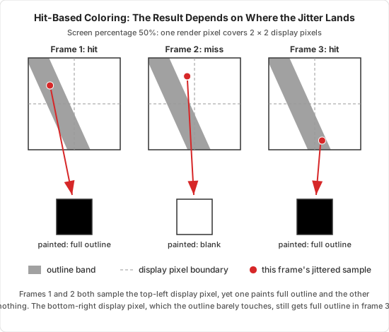
A better approach is to give each display pixel the same answer every frame, instead of one that depends on where the jitter happened to land. Given the frame’s jittered sample position, identify the display pixel it falls in. Then compute the fraction $c$ of that display pixel’s area covered by the outline, the band of the chosen thickness around the reconstructed line, and pass the alpha multiplied by that coverage to the painting shader:

Every sample that lands in a given display pixel now reports the same value, the average the upscaler would otherwise have to build up over many frames.

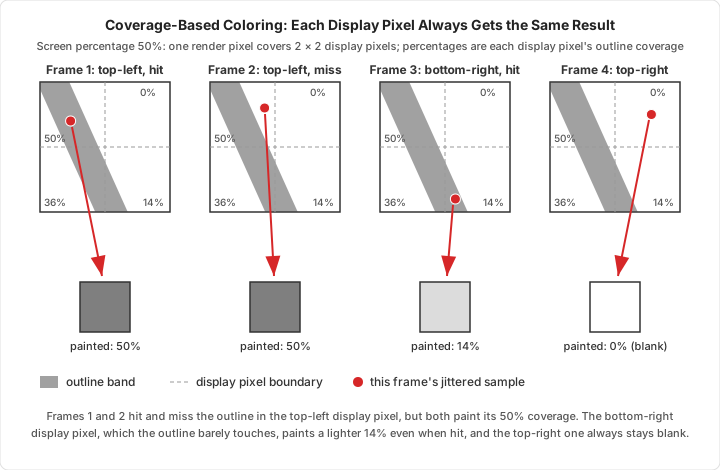
This significantly reduced the fading and blinking with TSR. The outline still faded intermittently in places, though.

Spatial Filter

The remaining fading came from a different kind of instability. Each render pixel reconstructs its own line segment from its own records, so the edges are temporally stable within each pixel, but not spatially stable across neighboring pixels. Where a contour passes from one pixel into the next, the two segments have slightly different slopes and intercepts and don’t quite meet. The coverage along the seam shifts as the records update, and the outline fades in and out there.

The fix is a spatial filter that blends each pixel’s line with the lines of its neighbors along the contour. It’s inspired by SVGF (Spatiotemporal Variance-Guided Filtering, Schied et al. 2017), an edge-avoiding denoiser for path tracing: like SVGF, it weights each neighbor by how uncertain its value is, and stops at geometric boundaries.

The filter runs as its own pass after every pixel has reconstructed its line, and only on pixels that contain an edge. For a target pixel $p$, it looks at all 8 neighbors in its $3\times3$ window. Which of them continue the edge depends on the edge’s slope, so the filter considers all of them and lets the weights decide.

For blending, each line is written in normal form, $\mathbf n \cdot \mathbf x = c$, with $\mathbf n$ the line’s unit normal and $c$ its offset from the pixel’s center. That form works for edges of any orientation, so lines from horizontal- and vertical-inducer pixels can be blended together. A neighbor $q$ at offset $\Delta_q$ from $p$ brings its line into $p$’s frame with $c’_q = c_q + \mathbf n_q \cdot \Delta_q$, flipping $\mathbf n_q$ first if it points against $\mathbf n_p$. Each neighbor then gets a weight made of five factors:

• Confidence. $\sigma_q^2$ is how uncertain $q$’s line position is at the edge of its pixel, where neighboring segments have to meet. It combines the position and slope standard errors of $q$’s reconstructed edge. A freshly reset record is very uncertain and barely counts.
• Continuity. $c’_q - c_p$ is how far apart the two lines are at $p$’s center. Pixels the edge actually runs through score close to zero, while a parallel edge one pixel over is about a pixel off and gets rejected. This is the term that makes the filter follow the edge.
• Direction. Compares the two lines’ orientations, so the filter doesn’t blend around sharp corners or where two edges cross, which the continuity term alone would let through.
• Depth. SVGF’s depth weight. It uses $p$’s depth gradient to predict how much the depth should change over the offset to $q$ if both sit on the same surface, and penalizes only the excess. Surfaces seen at a grazing angle aren’t cut apart, but occlusion boundaries are.
• Co-trigger. $\omega_q$ lowers the weight of neighbors whose records mix in a second edge.

A pixel only blends with neighbors of its own edge type, and silhouette pixels leave out the direction and depth factors, setting both to 1. Along a curved silhouette, the line legitimately turns with the surface, and every pixel of the edge stores the same smooth foreground depth, so neither factor carries useful information there. The target pixel takes part too, with its own confidence and co-trigger factors, and its new line is the weighted average of the lines’ normals and offsets. The outline intensity is blended with the same weights. Like SVGF, the filter also tracks how much each blend tightens the uncertainty, so it can be run more than once, each pass reaching one pixel further along the edge.

The filter reduced the fading noticeably, but it isn’t perfect. The result still depends on the screen percentage: the lower the percentage, the more the outline fades.

Note that the spatial filter runs before dense edge suppression, even though this post describes suppression first. Suppression only keeps dense edges from being painted in the final image.

Just Paint After TAA

The most thorough fix for the fading is to not hand the outline to the temporal upscaler at all: paint it at display resolution, after the TAA stage. Every problem in this section comes from painting a sub-render-pixel outline into render pixels and hoping the upscaler reconstructs it faithfully. The reconstructed lines don’t need that. They are continuous line equations, so they can be evaluated directly at each display pixel, with exact coverage, and the result no longer depends on the screen percentage or on how well the upscaler converges on thin features.

The catch is where TAA sits in the pipeline. In Unreal Engine, as in many renderers, TAA runs after translucency has been composited, so painting after TAA means painting on top of every translucent material and volume. An object standing inside fog, for example, would get a crisp outline drawn over the fog, as if the fog weren’t there. Fixing that would need to know how much translucency lies in front of each outline pixel, which is no longer available once everything has been composited.

Spatial Filter Improvement Ideas

If painting after TAA isn’t an option, here are two ideas I haven’t tried yet that might get the filter closer to removing the fading entirely.

Checking Connections Between Neighbors

The current kernel measures every weight against the target pixel’s own line: how far a neighbor’s line is from it, and whether the two point the same way. That’s a weak spot, because the target’s line is least reliable exactly where the filter is needed most, along a seam that’s fading or on a pixel whose record was just reset. A good neighbor can be rejected because the target’s line is off, and a stray neighbor can be accepted because it happens to agree with a wrong target line.

A better check compares the neighbors with each other. Take a neighbor A and extend its line across the kernel. If the extended line doesn’t pass through the target pixel, A’s edge doesn’t continue through the target, and A is discarded. Otherwise, follow it through the target to the neighbor B it reaches on the far side, and compare A’s line with B’s line and with the lines of B’s adjacent neighbors in the kernel. B’s neighbors are included because the cell the extended line lands in depends on the slope, and the edge may pass just beside B. If one of them matches, there is very likely a persistent edge running straight through the target, so A’s weight goes up, and so does the weight of whichever pixel matched on the far side.

The evidence for an edge through the target then comes from two separate records on opposite sides of it, instead of from the target’s own, possibly noisy line. The cost is extra comparisons: each neighbor is checked against up to three candidates on the far side, instead of just once against the target.

Silhouette Depth Factor

The current kernel turns the depth factor off for silhouettes. A silhouette is exactly where depth jumps, so comparing a silhouette pixel’s own depth with its neighbors’ mostly measures that jump, not whether the neighbors lie on the same edge.

The depth factor could still be used for silhouettes, as long as it’s based on the foreground surface instead of the silhouette pixel’s own: the foreground’s depth, fetched from the neighbor that is supposed to be the foreground, the one the pixel’s check fired against. Along a single silhouette, the foreground’s depth changes smoothly, so the factor passes. Where the silhouettes of two different foreground objects line up side by side, such as an arm in front of a torso, the foreground’s depth jumps, and the factor keeps the two outlines from blending into one. The depth gradient used for SVGF’s prediction would have to come from the foreground surface as well.

Limitation of the Algorithm

Sub-Pixel Details

The algorithm can only sample as finely as the G-buffer’s resolution. Every detection compares two samples one render pixel apart, and the reconstruction assumes each edge has a full pixel-wide band around it in which that comparison fires. Details smaller than a pixel, such as a thin wire, a small hole, or a narrow gap, break that assumption. The comparison only fires on the few frames where the two samples happen to straddle the detail, if at all, so the edges such details induce are reconstructed only partially, or not at all.

Statistical Noise

The reconstructed lines are statistical estimates, built from samples accumulated over time, so they always carry some variance.

• Estimates take time to converge. When an edge first appears, or a pixel’s history is reset by reprojection rejection, its record starts with only a handful of samples, and the reconstructed line wobbles until enough frames have accumulated. The standard errors from Edge Selection measure exactly this.
• The noise never reaches zero. The decay rate caps how many samples a record effectively holds, so even a fully converged record keeps some residual wobble. A slower decay gives a steadier line, but takes longer to recover after a reset and follows moving edges more sluggishly. A faster decay reacts quickly but stays noisier.
• Hard decisions amplify the noise. Each pixel makes yes-or-no decisions from these estimates, such as whether it contains the edge and which inducer’s edge to draw. Near a threshold, a little noise becomes a visible flip rather than a small wobble. Much of this post, from the 3rd approach to the reliability tests and the spatial filter, is about keeping that noise from turning into dashed or fading outlines.

How I Came Up with the Algorithm

I was working on outlines, and I started with a simple G-buffer algorithm: check the four axial neighbors of each pixel and decide whether to paint it with the outline. To make the result look thin, I blurred it.

Then I had an idea: record the extreme position, along the inducer’s axis, at which the G-buffer check detected the edge.

For the left inducer, I recorded the minimum $x$ at which the outline was detected, for the right inducer the maximum $x$, and for the vertical inducers the same with $y$. The outline was then painted only when the jittered sample position fell within that recorded range. I asked Claude Fable to implement it.

Of course, that only worked for axis-aligned edges. A single extreme along one axis can’t describe a slanted edge, so diagonal edges came out jagged.

So I went back to the blurring method, and then found that dense outlines flickered.

My first fix was to accumulate the outline’s strength over time, as an alpha value.

That made the outline worse and the jagging stronger: every jittered sample within a render pixel now produced the same result, so the upscaler had no sub-pixel detail left to reconstruct.

Next, inspired by the SVGF paper, I asked Fable to add a weighted temporal filter: a temporal estimator tracked the variance of each pixel’s outline alpha, and the filter was applied only to pixels with high variance. (This method is no longer used)

Then I came up with another idea.

I had been recording only the minimum or maximum along one axis. What if I recorded both the minimum and the maximum along the inducer’s axis, together with the other coordinate at the moment each occurred?

For the left inducer, say the detected position with the smallest $x$ so far was $(x, y) = (0.1, 0.2)$, and the one with the largest $x$ was $(0.8, 0.7)$.

I’d record both points. If a later sample detected the edge at $(0.9, 0.77)$, it would replace $(0.8, 0.7)$.

Those extreme points trace out the parallelogram-shaped region where the edge can be detected, and from that shape, the edge’s line segment itself.

To let stale records be replaced, new samples wouldn’t be compared against the recorded extremes directly. Instead, the recorded extremes would decay over time, the minimum creeping up and the maximum creeping down, so an old extreme would eventually lose to a fresh sample.

I asked Fable about this idea, and its answer came down to four points:

• A min/max record like this is statistically unstable.
• A single outlier can corrupt the record, and it may not be superseded for a long time.
• Why not use OLS regression instead?
• As in the SVGF paper, temporal accumulation can build unbiased estimators.

I was flabbergasted. I simply hadn’t thought of OLS regression, even though it’s something you learn in a first- or second-year university statistics course.

Fable didn’t hand me a brilliant idea out of nowhere. It filled a hole. But that hole was in a critical, load-bearing part of the idea, and it had been making everything else creak.

Looking back, it went like this:

1. When I first came up with the min/max idea, Fable didn’t point out any problem with it.
2. In a later session, I gave Fable, or reminded it of, the knowledge of temporal estimators, with the SVGF paper as a reference.
3. I came up with the idea of recording the points with the minimum and maximum values along the inducer’s axis.
4. Fable finally came up with the fix for the critical problem in my idea.

References

Christoph Schied, Anton Kaplanyan, Chris Wyman, Anjul Patney, Chakravarty R. Alla Chaitanya, John Burgess, Shiqiu Liu, Carsten Dachsbacher, Aaron Lefohn, and Marco Salvi. 2017. “Spatiotemporal Variance-Guided Filtering: Real-Time Reconstruction for Path-Traced Global Illumination.” In Proceedings of High Performance Graphics (HPG ‘17). ACM. https://doi.org/10.1145/3105762.3105770

How to Cite

If you reference this post, please cite it as:

Donguk Lim. “TAA-Compatible Toon Outlines: The Pixel-Thickness Problem with G-Buffer Contours.” Notes on Rendering (blog), September 6, 2026. https://donguklim.github.io/rendering/npr/2026/09/06/taa-compatible-toon-outline-gbuffer-contour.html

Or in BibTeX:

@misc{lim2026taatoonoutlines,
  author       = {Donguk Lim},
  title        = {{TAA}-Compatible Toon Outlines: The Pixel-Thickness Problem with {G}-Buffer Contours},
  howpublished = {Notes on Rendering (blog)},
  year         = {2026},
  month        = sep,
  url          = {https://donguklim.github.io/rendering/npr/2026/09/06/taa-compatible-toon-outline-gbuffer-contour.html}
}